One of the most enigmatic parts of pump operation is how performance changes
when pumps are driven by Variable Frequency Drives (VFDs). Unfortunately, many
people who operate them (and quite a few who select them) don’t have a good
understanding of how they work as system conditions and demands fluctuate. Make
no mistake, most system conditions vary constantly as levels, usage, and even
the pumps themselves slowly change. The affinity laws govern how pumps react to
these changing conditions.
Constant or variable speed
Pumps operate in two configurations: constant speed or variable speed. A constant speed pump is driven by a motor typically supplied by the local mains electricity (or a higher voltage equivalent if it’s a really big motor and pump). However, you can also add a VFD to the setup. While slightly more inefficient than a direct mains connection, VFDs add the ability to modulate an AC electric signal. In the US, the electric grid is a 60 Hz waveform. The VFD can simulate electric wave patterns at a wide range of frequencies which physically spin the motor at a different rate.As you might predict, pumps don’t move liquid identically when motor frequency changes. First, let’s look at a basic pump curve:
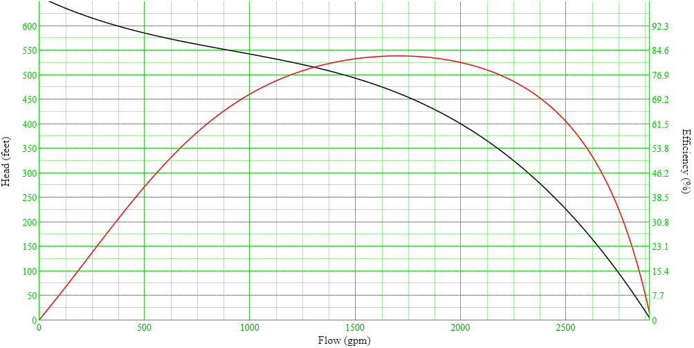
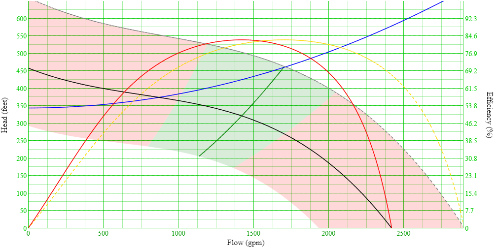
A pump curve (in black) shows how much liquid the pump will move at a given head. Head is just the difference in pressure across the pump. There’s also an efficiency curve (in red), which shows how efficiently the shaft energy from the motor is transferred to the water. For the above curve, if the pressure in front of the pump was 400 feet higher than the pressure behind the pump, it would produce 2000 gallons per minute of liquid at 80.6% efficiency. To determine where a pump would operate in a given system, an engineer calculates the system response to a given flow rate (specifically, how much friction loss there is in the system) and overlays this on the pump curve. This is called the system curve:
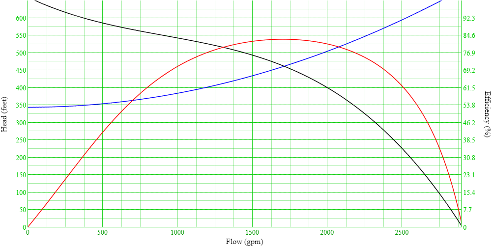
The pump will operate at the intersection of the pump curve and system curve (in blue). In the above example, this is at 462 feet of head and 1715 gpm at 82.9% efficiency. A constant speed pump only has this head curve available and will track up and down it as the system curve changes. A variable speed pump, though, has a range of potential operating points. The affinity laws tell us that the flow produced by the pump changes linearly with speed, head changes with the square of speed, and the power consumed changes with the cube of speed. Mathematically, that means:
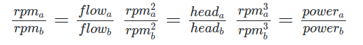
To find a point on the scaled curve, multiply the full speed flow by the speed ratio and the full speed head by the speed ratio squared. If a pump slows to 55 Hz from 60 Hz, the new pump curve looks like this:
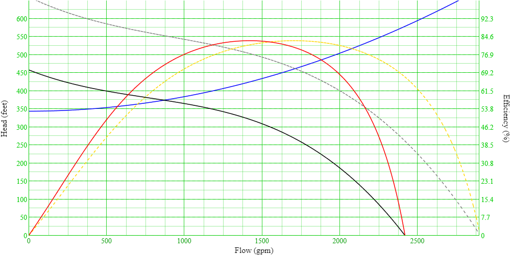
Based on the previous system curve, the pump would now produce 871 gpm at 374
feet of head at an efficiency of 72.5%. Seemingly small changes in speed produce
very large changes in operation. In this example, the pump stops producing a
flow when speed reaches 43 Hz.
Most operators and engineers aren’t getting this sort of feedback on their
pumps. Most pump stations have one flow meter for a bank of pumps and the
calculated system curves are out of date or entirely unknown. What makes this so
important is the Preferred Operating Range (POR). The POR is a range of flows
measured from the pump’s Best Efficient Point (BEP) and pump manufacturers
recommend that pumps be operated within POR at all times. Here’s the pump with
the POR overlaid:
A seemingly innocuous change of slowing the pump down to 50 Hz made the pump operate much less efficiently and outside of POR. However, sometimes slowing the pump down can make the pump operate more efficiently too! It depends on the system curve, the pump curve, and the current system demands. The only way to correctly operate pumps is to track operation and compute pump flow and head in real time. Until then, a little more understanding about changing hydraulics can help gain some insight into what is happening. You can do that by playing with this interactive demo:
