Scheduling Pump Repairs using Financial Metrics
How I Learned to Stop Worrying and Avoid Run-To-Failure
Most pump maintenance at water and wastewater utilities is not planned. A commissioned, operating pump is largely left alone as long as it keeps working. Even if a pump is operated perfectly, it will eventually wear out and gradually become less efficient. Chances are it will stay in service well after its useful life has ended. At some point, someone notices that the pump isn’t keeping up with demand or it will suffer a catastrophic failure. In either case, maintenance on the pump is not something scheduled or predicted; it is a crisis. This practice is called “Run-To-Failure.”
With most current control and monitoring systems, there’s not a whole lot else utilities can do. They don’t really know what state their pumps are in, they don’t know where those pumps are operating, and they don’t know how they should be controlling their pumps. Pump health is an enigma and, lacking the right data to forecast repairs, utilities react to problems as they come up. No one wants to use a pump that can’t contribute. No one wants to waste money running inefficient pumps. No one wants to run their pumps to failure. It’s a reliability and financial concern that many utilities see as the state of the art.
Intelligent Pump Management
However, there are better ways to run pump stations and manage pump repairs using Intelligent Pump Management. Using historical station data, we can calculate how much energy worn pumps are costing a utiltiy. Coupled with some basic economic factors, we can turn these energy costs into actionable financial metrics that tell us when to pull the trigger on pump repairs. There are some prerequisites, though. First, you need current, accurate test curves for each pump in a pump station (for more on test curves, check out this rabbit hole). Second, you need Specific Energy Maps to plot out what the station is capable of at a given set of system demands and pressures (for more on SEC maps, check out this other rabbit hole).With tested pump curves and Specific Energy Maps, the full potential of a pump station is unlocked. By correlating these maps with operating history, you can compute how much each worn pump is costing the utility at a given point in time. For instance, let’s say we have a pump station with five variable speed pumps (if you want to learn more about variable speed pumps, I have one more rabbit hole). In this example, we want to know how much energy we could save by repairing pump 2, the oldest pump in the station. We start going through the historical operation of the station and find that we were running at 1630 gpm for an hour last week. Using our SEC Map solved for that set of system conditions, we want to find the most efficient way to achieve that flow with the current set of pumps:
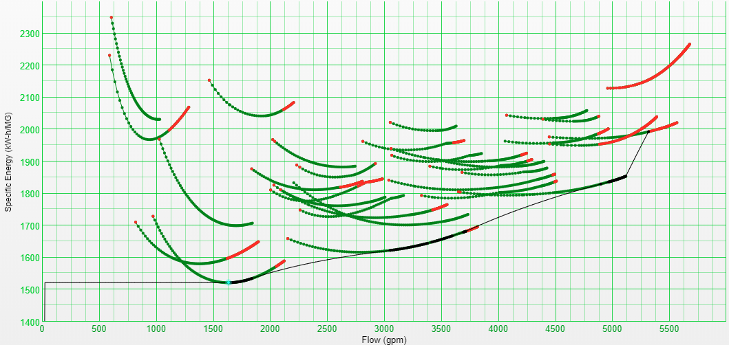
The best way the station can operate at 1630 gpm is at a specific energy consumption of 1521.6 kWh/MG at the cyan point. During that hour, the current pumps would produce 98,040 gallons of water and use 149.2 kWh to do it. Next, to see if pump 2’s state is hurting the utility, we need another map with the same system conditions, but with pump 2 replaced with a factory new pump:
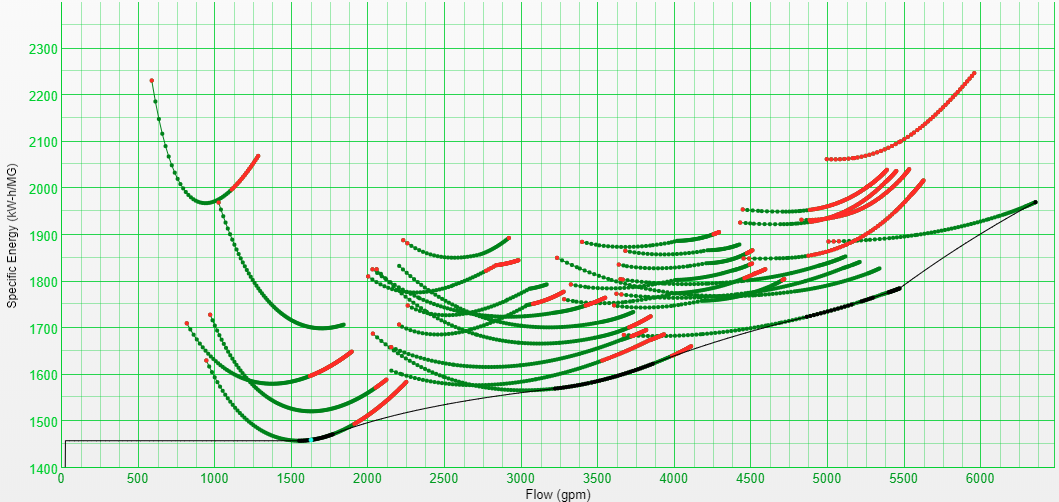
Replacing pump 2 would allow the station to hit this flow at a specific energy consumption of 1460.3 kWh/MG. So, the station would produce the same 98,040 gallons of water but only consume 143.2 kWh to do it. That’s a savings of 6 kWh for the hour.
Next, repeat this comparison at each different operating point in the past year. Finally, total all these energy deltas to calculate the annual energy reduction for the pump repair. That’s the whole process. It’s simply calculating how efficient the pump station could have been with a new pump.
This process needs to be done for each pump by itself so we can see how much each worn pump is costing us independently. Once we have this annual energy reduction for each pump, we need our economic factors:
-
Annual Discount Rate: The cost of money. Also called an interest rate. This is effectively how much we prefer current money over future money. We’ll be using 3% for our calculation, which is pretty standard.
-
Expected Pump Life: How many years we want to take credit for energy savings. We’re using 10 years.
-
Energy Cost: Average energy cost in $/kWh. We’re using 0.1 $/kWh
-
Pump Repair Cost: The soup to nuts, all-in cost of pulling the old pump, buying a new pump or repairing the old pump, and putting the new pump in the ground. This might be different for each pump.
With these inputs, we can treat the annual energy reduction as an annuity and calculate the following:
-
Net Present Value (NPV): The difference between an investment cost and the ‘present value’ of its dividends. In our case, the pump repair cost versus the present value of the resultant energy savings. A positive NPV means the investment generates money.
-
Return on Investment (ROI): The net gain from an investment divided by the investment cost. Usually expressed as a percentage, the ROI shows the relative efficiency of an investment (how much bang you get for your buck).
-
Internal Rate of Return (IRR): The calculated discount rate that would make the NPV of a project $0. It shows at what rate the project would break even.
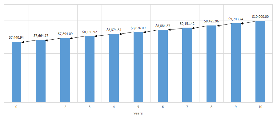
All of these metrics depend upon the ‘present value’ of the annual energy savings. Finding the present value of the annuity means we are depreciating each year’s savings by the discount rate because money in the future is worth less than money now. For example, one single payment of $10,000 ten years in the future has a present value of $7440.94. It is discounted by our 3% each year like this:
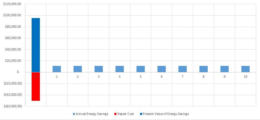
In our example, repairing pump 2 would save 111,580 kWh per year, or $11,158 per year. We discount each future energy savings back to the current year and then sum them all together to get its present value. Using a pump life of ten years, the present value of those savings looks like this:
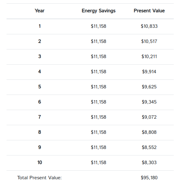
Finally, subtract off the repair cost and you are left with the Net Present Value of the pump repair. If your NPV is positive, it means you will save money through the repair:
After we have run this analysis for each pump, the data looks like this:
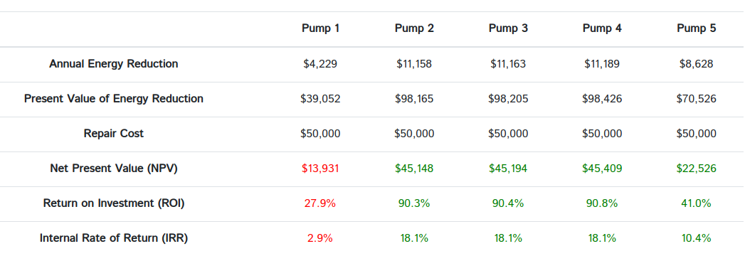
All that’s left is to compare the NPVs across the pump station. Several pumps have positive NPVs, meaning the pump repair would pay for itself in energy savings. However, we would recommend repairing pump 4 since it has the highest NPV (albeit by a small margin). The takeaway from this table is that it is in the owner’s best economic interest to repair pump 4. Leaving the pump in service is going to cost the utility more money. Additionally, repairing or replacing the worn pump has other benefits, like increased station capacity and reliability, which we aren’t trying to quantify here. Also note that pump 1, the newest, healthiest pump, has a negative NPV.
Please note that these NPVs across the station are not additive. Each is only good for a single pump repair. If pump 4 is repaired, the other calculated NPVs are invalid because the baseline energy performance of the pump station has changed. However, you can run a new solve with that new baseline and see if it makes economic sense to repair another pump.
Pumps no longer need to be run to failure. It is an old, terrible way to do things. This process allows utilities to keep their pump stations in better condition and save money while doing it. With a little data and some analysis, it’s possible to turn this handy wavy standard into a crisp, clean financial decision. It helps make the water production industry a little safer, a little more efficient, and a lot more tractable.